Database internals (part 1): notes on storage engines and PostgreSQL
At work we need to improve the ingestion of a Timeseries database. We tried PostgreSQL + TimescaleDB but unfortunately we're only achieving ingestion from ~700 IoT devices in our benchmarks.
It's time then to become somewhat of an expert of PostgreSQL and TimescaleDB; for doing good optimization I need to know the internal architecture and details of the software.
These are notes I've gathered from different sources. Writing them out helps me learn better, and they're handy to look back on.
Disclaimer
This article is a collection of educational notes and summaries based on the copyrighted sources listed below. For complete and authoritative information, please refer to the original works. Images and substantial passages are derived from the cited sources under fair use for educational purposes.
This compilation and original commentary are offered for personal learning and reference. For any complaints, please contact me.
Resources
The following works served as the primary sources for this article:
- The Internals of PostgreSQL - Hironobu SUZUKI
- Designing Data-Intensive Applications - Martin Kleppmann
Complementary data and analysis were generated or enhanced using Claude models.
Theory
Indexes
Indexes are auxiliary data structures that speed up data retrieval by avoiding full table scans; the choice of index type determines the trade-offs between read performance, write overhead, and supported query patterns.
Hash Indexes
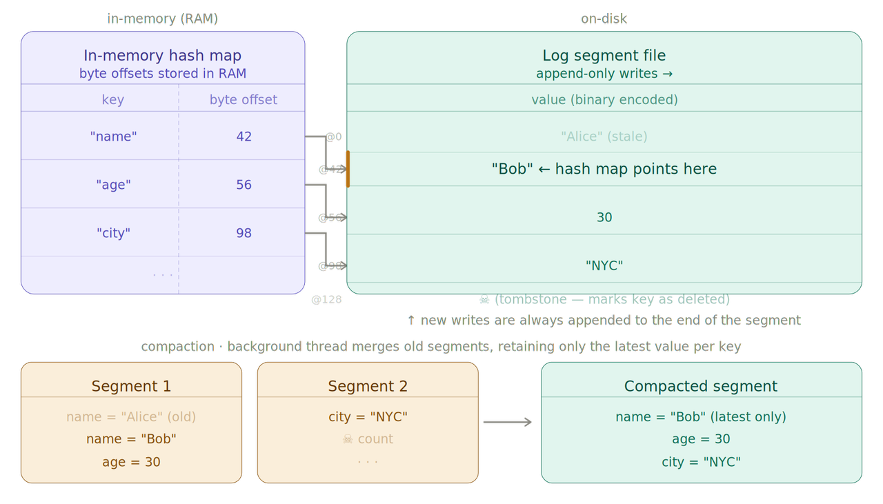
Keep an in-memory hash map that maps each record key to the byte offset of its value in the on-disk log file.
The new writes are always appended. In order to avoid running out of disk space we break the log into segments files. When the segment reaches a certain size or retention then a compaction procedure is run where we keep only the latest value for each key.
In order to avoid blocking the read/writes we can merge old segments with a background thread which will write to a new segment.
Some characteristics of this approach:
- the key cardinality should not exceed ram size
- read/writes can be really fast thanks to Caching. If the page is in cache then virtually no I/O operation is needed.
- usually values are encoded with a binary format into the file
- tombstone records are used to delete records.
- crash recovery is handled by replaying the segments and using checksum for partial written records or some types of optimizations starting from there
- write is strictly sequential so usually a single thread is used while reading can be concurrent.
- range queries are not efficient. you have to scan the entire hash index
SSTables
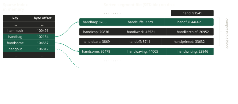
Rather than appending data and maintaining a complete Hash Index, Sorted String Tables keep segments ordered by key and use a sparse index.
This gives us the following properties:
- When merging segments we can use mergesort
- We don't have O(1) read access but we have O(n/m) where n is the number of elements in the segment and m the cardinality of the sparse index for the segments; or O(log(n/m)) when the subsegment has key+value with a fixed size
- Each subsegment can be compressed to limit I/O
LSM-tree
How do you get data sorted in the first place? Two ways:
- Structure on disk
- In memory data structure
For LSM-trees we use an in-memory data structure, in particular balanced tree data structures like AVL-trees or red-black-trees.
So the flow is like this:
- When a write come in, add it to the balanced tree (also called memtable). This operation has a complexity of O(log(n))
- When a retention policy (size or time) is reached we write to disk the memtable as an SSTable. Given the already ordered balanced tree this operation can be done efficiently and in background.
- When serving a read request, first we try to find it in the memtable and then we iterate over each SSTable in the disk. This operation is very expensive when the entry is not present. An optimization is to maintain a bloom filter to end the read request in O(1) when the key is not present.
- Run compaction background threads from time to time
The main problem of LSM-tree is that in case of crash we lose the balanced tree data structure in memory.
B-Trees
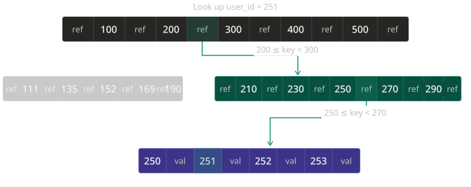
B-Trees keep key-value pairs sorted by key but it does it directly on disk.
B-trees break the database down into fixed-size blocks or pages to align better with the underlying file-system and hardware.
Each page can be identified using an address or location which is used to construct a tree of pages. The number of references to child pages in one page is called branching factor.
The B-tree with n keys is always balanced and has always a depth of log(n) meaning that a search for a value is O(log(n)).
Usually the depth is 3/4 levels. (A four-level tree of 4KB pages with a branching factor of 500 can store up to 250TB)
Overwriting values in place on disk means that the operation is not immune to crashes. In order to make the database reliable to crashes, it's common to include an additional data structure on disk: a write-ahead log (WAL or redo log). This is an append only file to be written before each operation on the B-tree. The log is used for restoring after the crash to a consistent state.
Additional care must be taken when multiple threads are going to access the B-tree at the same time. This is typically done by protecting the tree's data structure with latches (lightweight locks).
Log-structured approaches are simpler in this regard, because they do all the merging in the background without interfering with incoming queries and atomically swap old segments for new segments from time to time.
Comparing LSM-trees and B-trees
As a rule of thumb LSM-trees are faster for writes, whereas B-trees are thought to be faster for reads.
The main advantages of LSM-trees is the lower write amplification and less fragmentation.
The main downside is that you have to carefully configure the compaction operations. If not set up carefully, the operation might not keep up with the rate of incoming data.
B-trees also are attractive in databases that want to offer strong transactional semantics thanks to locks directly attached to the tree.
Other Indexing Structures
Since secondary indexes permit duplicate keys while B-tree leaves enforce uniqueness, a reconciliation strategy is needed. Two solutions exist:
- Appending record number to the key:
key->new_key=(key,row_id) - Each value in the index is a list of row ids:
key->list[row_id]
Secondary indexes, of course, are part of the picture too. This raises a key question: how do we store them without duplicating data?
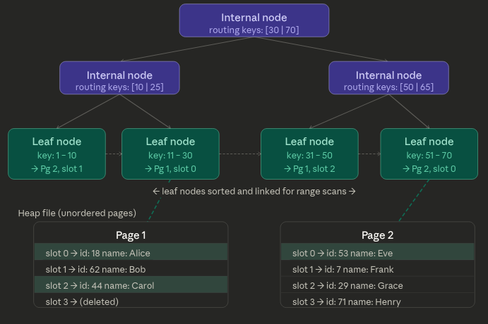
When using B-trees the leaf nodes point to heap file. A Heap file is an unordered collection of pages, where each page holds a bunch of records. So with B-trees the heap file corresponds to the record in the key range.
The Heap file approach is common because it avoids duplicating data when multiple secondary indexes are present: each index references a location in the heap file and the actual data is kept in one place.
The update in place of values without changing a key is efficient provided the new value is not larger than the old one. For the latter case we need to update all the references to the new position or use a forwarding pointer to the new heap location.
In some situations, the extra hop from the index to the heap file is too much of a penalty so it can be desirable to store the indexed row directly within an index.
This is known as clustered index. Then secondary indexes can refer to the primary key which makes the read operation O(2log(n))~=O(log(n))
A compromise between a clustered index and a nonclustered index is known as covering index, which stores some of a table's columns within the index. Some queries then can be optimized to use only the covered columns.
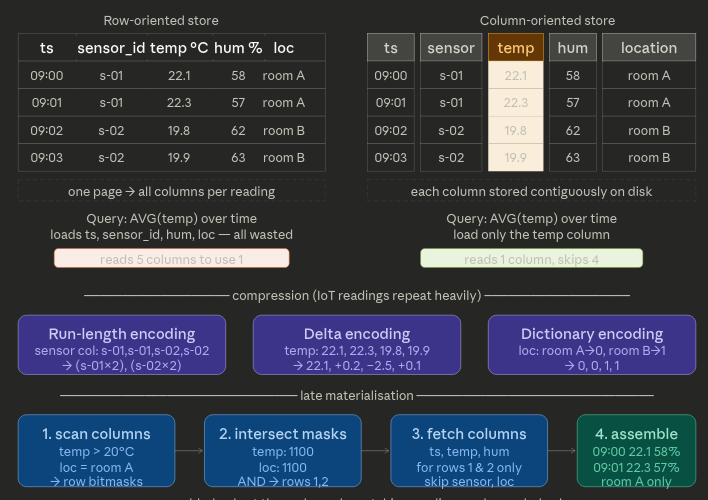
Column Oriented Storage
If you have to store petabytes of data storing them and querying them becomes difficult. Most of the time, queries only access 4 or 5 columns. We can execute the query effiently by using column oriented storage.
The idea behind it is simple: don't store all the values from one row together, but store all the values from each column together instead.
If each column is stored in a separate file, a query only needs to read and parse those columns that are used in that query, limiting I/O.
Also compression can reduce the I/O bandwidth further, and using compression on column data with a low entropy can save more disk space. Different compression techniques are used, such as:
- bitmap encoding (useful when the cardinality of the values is low)
- run-length encoding, dictionary encoding, and other compression techniques
Replication
The difficulty handling replication is caused by the changes on the replicated data.
There are three popular algorithms for replicating changes between nodes:
- Single-leader
- Multi-leader
- Leaderless replication
Replication exists in two flavours:
- Synchronous
- Asynchronous
Simply put, when replication is synchronous the master node responds "okay" to the user/process only after receiving the "okay" from the slave node, while in asynchronous replication the master's acknowledge is sent immediately after having written the change to its persistence.
Different replication methods exists:
-
Statement-based replication: the leader logs every write request and sends those to its followers. This means that every follower parses and executes those SQL statements.
It has problems with autoincrementing and nondeterministic queries. It's not used a lot.
-
Write-ahead log shipping: in the case of a log-structured engine (SSTables or LSM-Trees), this log is the main place for storage. In the case of a B-Tree then the log in question is the write-ahead log. In either case, the log is sent to the followers which build the exact same data structure found on the leader.
The main disadvantage is that the log describes the data on a very low level: a WAL contains details of which bytes were changed in which disk blocks. This makes replication closely coupled to the storage engine. This can be a problem when upgrading nodes because it might not be possible to run different versions of the database software.
-
Logical (row-based) log replication: the idea is to use a logical log which is a sequence of records describing writes to database tables at the granularity of a row. A transaction that modifies several rows generates several such log records, followed by a record indicating that the transaction was committed. This technique is also called change data capture.
Transactions
The safety guarantees provided by transactions are described by the acronym ACID, which stands for Atomicity, Consistency, Isolation and Durability.
In practice, one database's implementation of ACID does not equal another's implementation. For example, there's a lot of ambiguity around the meaning of Isolation.
Atomicity means that a transaction composed of multiple writes has two possible outcomes: every write is completed and the transaction is committed or if anything goes wrong the transaction is aborted and no modification has happened on the database.
Consistency idea is that you have certain statement about your data (invariants) that must always be true. If a transaction starts with a database that is valid according to these invariants, and any writes during the transaction preserve the validity, then you can be sure that the invariants are always satisfied. However, this idea depends on application's notion of invariants, and it's the application's responsibility to define its transactions correctly so that they preserve consistency.
Isolation means that concurrently executing transactions are isolated from each other: they cannot step on each other's toes. There are various levels of isolation. The strongest one is Serializable that is the equivalent of the transaction running serially even if they run concurrently. More on isolation later.
Durability in single-node DBs means that the data has been written to nonvolatile storage, while for replicated DBs it means that the data has also been copied to some number of nodes.
Isolation Levels
Databases have long tried to hide concurrency issues from application developers by providing transaction isolation.
Serializable isolation means that the database guarantees that the transaction have the same effect as if they ran serially. In practice, Serializable isolation has a performance cost, and many databases don't want to pay that price. It's therefore common for systems to use weaker levels of isolation, which protect against some issues, but not all.
First Level: Read Committed
The first level is Read Committed which makes two guarantees:
- No dirty reads: when reading you will see only committed transactions.
- No dirty writes: it's possible to overwrite only data that has been committed.
This level does not prevent concurrency problems but guarantees the basics for having transactions.
Most commonly, databases prevent dirty writes by using row-level locks while for dirty reads, old values are kept during the uncommitted transaction and are returned as result for the read-query.
This level suffers from the read skew problem which occurs when a transaction reads data at different points in time, seeing some values before and some after another concurrent transaction commits, resulting in an inconsistent view of the database.
For example, imagine a transaction that is generating a report by summing up inventory across multiple warehouses. It reads warehouse A first (100 units), but before it reads warehouse B, a concurrent transaction moves 50 units from B to A and commits. The report transaction now reads warehouse B's already-updated value (50 units fewer), while having read warehouse A's old value, missing those 50 units entirely and producing an incorrect total.
Second Level: Snapshot Isolation
To fix the read-skew problem we need repeatable reads; Snapshot isolation is the most common solution to this problem.
The idea is that each transaction reads from a consistent snapshot of the database, which means that the transaction sees all the data that was committed in the database at the start of the transaction. Even if the data is subsequently changed by another transaction, each transaction sees only the old data from that particular point in time.
Snapshot isolation is useful for backups, analytics and integrity checks and is supported by PostgreSQL, MySQL and others.
To implement snapshot isolation it's usually used a generalization of the mechanism explained before to prevent dirty-reads.
The database must potentially keep several different committed versions of an object, because various in-progress transactions may need to see the state of the database at different points in time. Because it maintains several versions of an object side by side, this technique is known as multi-version concurrency control (MVCC).
In PostgreSQL, for example, when a transaction is started, it is given a unique, always-increasing transaction ID. Whenever a transaction writes anything to the database, the data it writes is tagged with the transaction ID of the writer. Each row in a table has a created_by field, containing the ID of the transaction that inserted this row into the table and a deleted_by field (initially empty) which contains the ID of the transaction which deleted the record. An update is instead treated as a deleted + create.
How do indexes work in MVCC DBs? An option is to have the index point to all the versions of an object and delegate the responsibility to the index query to filter out object versions not visible to the transaction. Later, a garbage collector can remove old versions. In practice, many implementation details determine the performance of MVCC.
For example, PostgreSQL has optimization for avoiding index updates if different versions of the same object can fit on the same page.
Many databases call snapshot isolation by different names: Oracle calls it "serializable", PostgreSQL and MySQL call it "repeatable read". And to top it off, IBM DB2 uses "repeatable read" to refer to serializability.
The snapshot isolation also needs to handle the lost update problem (the classic two parallel counter increments). Databases provide different solutions to this problem but most of these solutions require careful application-level discipline. The main solution are:
-
Atomic write operations: usually implemented by taking an exclusive lock on the object when it's read so that no other transaction can write it (or take a competing lock) until the update has been applied.
Unfortunately, object-relational mapping frameworks make it easy to accidentally write code that performs unsafe read-modify-write cycles instead of using atomic operations.
Example query which is concurrency-safe in most databases:
UPDATE counters SET val = val + 1 WHERE key = 'foo'; -
Explicit locking: simply lock objects that are going to be updated. Then the application can perform the read-modify-write cycle.
BEGIN TRANSACTION; SELECT * FROM inventory WHERE order_id = 1234 FOR UPDATE; -- The FOR UPDATE clause indicates that the database should take a lock on all rows returned by this query. UPDATE inventory SET stock = stock - 1 WHERE order_id = 1234 AND key = 'foo'; UPDATE inventory SET stock = stock - 1 WHERE order_id = 1234 AND key = 'bar'; COMMIT; -
Compare and Set: in databases that do not provide transactions, compare-and-set operations are sometimes available. The idea is simple: only perform the update if the value has not changed since you last read it. If it has, the update fails and you must retry.
-- You read the current value first SELECT stock FROM inventory WHERE product_id = 3; -- stock = 10 -- Then update only if the value is still what you read UPDATE inventory SET stock = stock - 1 WHERE product_id = 3 AND stock = 10; -
Automatically detecting lost updates: the idea is to let the updates run in parallel and, if the transaction manager detects a lost update, abort the transaction and force it to retry its read-modify-write cycle. PostgreSQL, Oracle and SQL server snapshot isolation levels automatically detect when a lost update has occurred and abort the offending transaction. MySQL InnoDB, by contrast, does not detect them.
There are other kinds of subtler race conditions that can occur when different transactions concurrently try to write to the same objects like Write Skew and Phantoms.
Write Skew is like a generalization of the lost update problem but sneakier. Instead of two transactions writing to the same object, they read the same data, make a decision based on it, and then write to different objects. No dirty read, no lost update yet the result violates a business constraint.
Classic example: Doctors on-call
Rule: at least 1 doctor must be on call at all times.
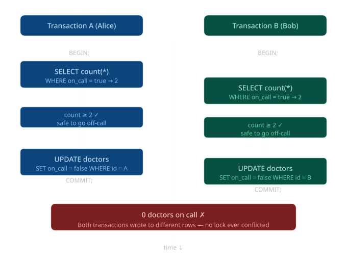
Here the problem could be solved using some techniques like the FOR UPDATE clause.
What makes this case particularly tricky is that it slips past snapshot isolation undetected. Because each transaction modifies a different row, one for Alice and one for Bob, there is no write conflict to speak of. Snapshot isolation is only concerned with two transactions touching the same object; since that never happens here, both writes are accepted cleanly.
The pattern always follows this shape:
- A
SELECTreads some shared state - Application code makes a decision based on that read
- An
UPDATEchanges a different object based on that decision - The invariant (at least 1 doctor on call) is now broken
Instead, a Phantom occurs when a transaction's query would return different rows if re-executed, because another transaction inserted or deleted rows in between.
-- Transaction A checks: is there any room in the meeting?
SELECT count(*) FROM bookings WHERE room_id = 5 AND slot = '14:00';
-- returns 0
-- Transaction B does the exact same check concurrently → also 0

-- Both decide it's safe to book:
INSERT INTO bookings (room_id, slot, user_id) VALUES (5, '14:00', 'alice');
INSERT INTO bookings (room_id, slot, user_id) VALUES (5, '14:00', 'bob');
-- Room is now double-booked ✗
The tricky part here is that SELECT FOR UPDATE doesn't help: there are no existing rows to lock when both transactions check. The row that causes the conflict doesn't exist yet at the time of the check.
The solutions are:
- Serializable isolation: the only level that fully prevents those problems
- Materializing the conflict: artificially inserting a lock row before it exists (e.g. pre-populate a slots table so there is always a row to lock with FOR UPDATE)
- Application-level constraints: like a UNIQUE index on (room_id, slot) that causes one of the inserts to fail
Third Level: Serializable
Serializable is the strongest isolation level. It guarantees that even though transactions may execute concurrently, the end result is identical to some serial execution. It fully prevents dirty reads, non-repeatable reads, phantoms, and write skew.
There are three main approaches:
-
Actual Serial Execution: it works in practice when transactions are very short and the dataset fits in memory (no slow disk I/O). Redis and VoltDB use this approach. The idea was that modern CPUs are fast enough that a single-threaded loop can outperform a multi-threaded system drowning in lock contention. (Did you say KISS?)
-
Two-Phase Locking (2PL): is the traditional approach. Several transactions are allowed to concurrently read the same object as long as nobody is writing to it. But when a transaction needs to write an object, exclusive access is required.
-
Serializable Snapshot Isolation (SSI): the modern approach. The best of both worlds: optimistic concurrency with full serializability. The idea is to let transactions run freely under snapshot isolation, but track dependencies between them. If the database detects that the combined outcome could not have happened in any serial order, it aborts one of the transactions.
The huge advantage over 2PL is that readers never block writers and writers never block readers: conflicts are only detected at commit time, not during execution. This gives much better throughput under high concurrency.
PostgreSQL Internals
In PostgreSQL, tables, indexes, sequences, views and functions are all database objects that are logically separated from each other and belong to their respective databases.
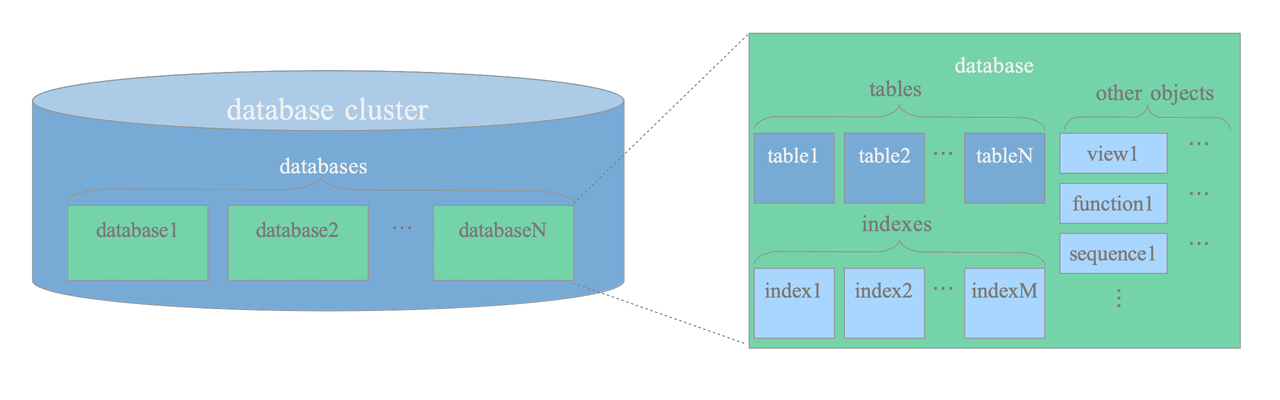
All DB objects are managed via object identifiers (OIDs) which are uint (4 bytes).
The relationship between objects is stored in system catalogs. System catalogs are the place where a relational database management system stores schema metadata, such as information about tables and columns, and internal bookkeeping information. PostgreSQL's system catalogs are regular tables.
Physical Structure of DBCluster
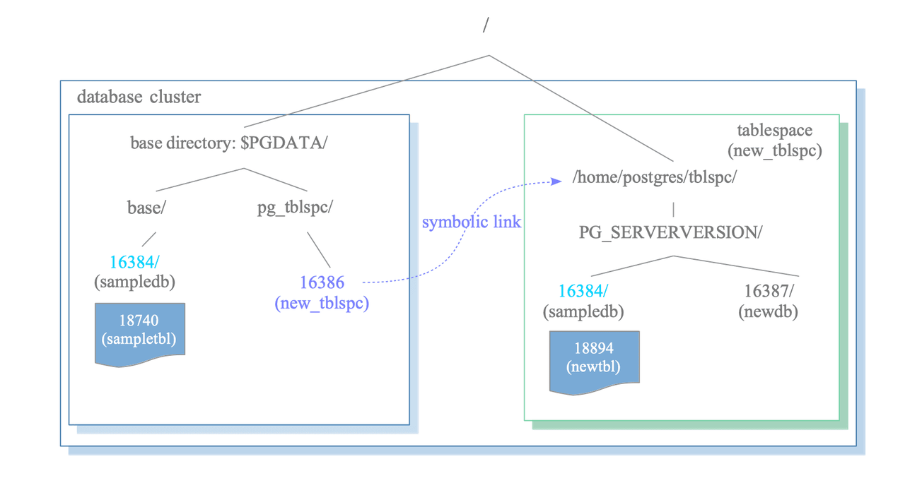
Postgres saves all configs, databases, etc. under $PGDATA as files; it also supports tablespaces but their meaning is different from other RDBMSs.
A tablespace in PostgreSQL is a single directory that contains some data outside of the base directory.
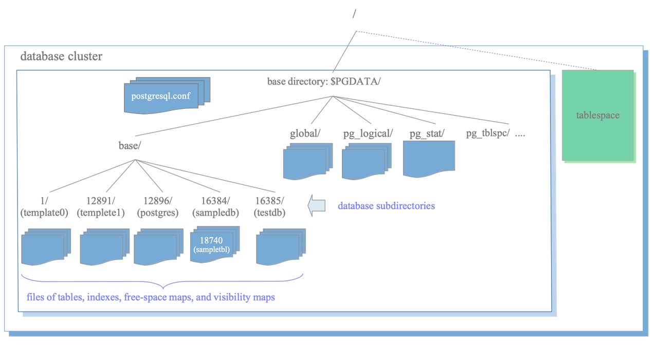
Tablespace is useful in two cases: when you want to spread data across different physical drives for performance (e.g. indexes on NVMe, cold data on slow disks), or when your main filesystem is full and you need to overflow onto another mount point.
The most important subdirectories are:
- base: Subdirectory containing per-database subdirectories.
- pg_wal: Subdirectory containing WAL (Write Ahead Logging) segment files.
- pg_xact: Subdirectory containing transaction commit state data.
- pg_multixact: Subdirectory containing multitransaction status data. (used for shared row locks)
- pg_commit_ts: Subdirectory containing transaction commit timestamp data.
Layout of Files Associated with Tables and Indexes
Each table or index whose size is less than 1GB is stored in a single file under its database directory.
Tables and indexes are internally managed by OIDs, while their data files are managed by relfilenode. The relfilenode values usually but not always match the respective OIDs.
When the file size of tables and indexes exceeds 1GB, PostgreSQL creates new files named like relfilenode.1 (..n) and so on.
Each table has two associated files, suffixed with _fsm and _vm. These are referred to as the free space map and visibility map, respectively.
The free space map stores information about the free space capacity on each page within the table file, and the visibility map stores information about the visibility of each page within the table file.
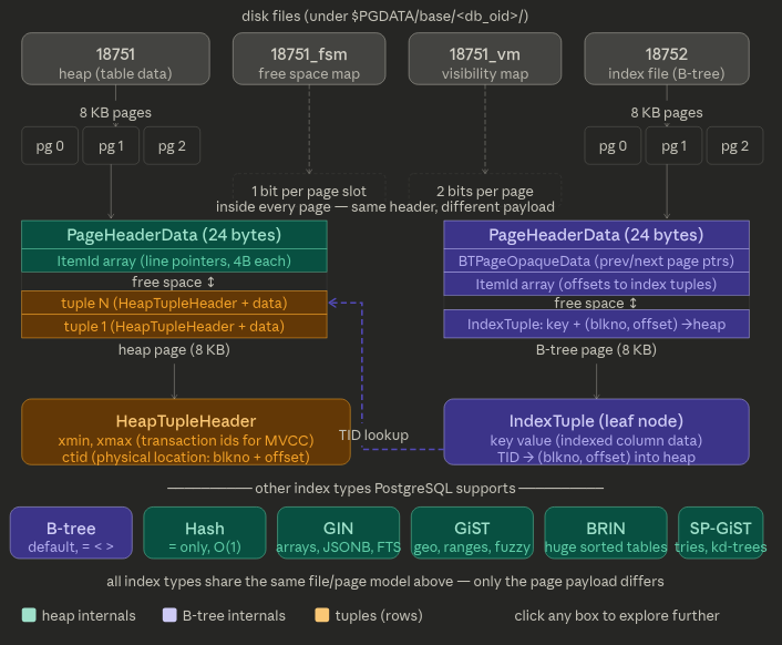
PostgreSQL's default index is a B-tree (technically a B+ tree variant), but it's just one of several index types it supports. Every file, whether a heap or an index, is split into 8KB pages, and the page format differs depending on what's inside.
Every file is just an array of 8KB pages. Whether it's a heap file (18751) or a B-tree index (18752), the physical format is identical at the outer level, a sequence of fixed-size pages. What differs is the payload inside each page.
The _fsm fork is how INSERT finds space fast. Without it, Postgres would have to scan pages looking for a free slot. The FSM is a compact tree of free-space fractions; it lets Postgres jump directly to a page with enough room for the new tuple.
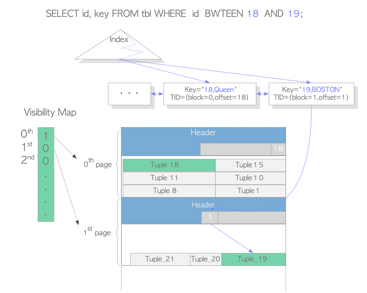
The B-tree leaf node stores a Tuple ID (TID), not the actual row. Each index entry is (key, TID) where TID = (block number, slot offset).
That's why after an index lookup you still need a second I/O to fetch the actual tuple from the heap.
PostgreSQL supports covering indexes.
-- multi-column: all three columns are part of the key (multi-column index)
CREATE INDEX ON employees (department_id, name, salary);

-- covering with INCLUDE: only department_id is the key
CREATE INDEX ON employees (department_id) INCLUDE (name, salary);
With INCLUDE, the non-key columns don't bloat the internal B-tree nodes, they only exist in the leaf nodes.
You can confirm an index-only scan is happening with EXPLAIN:
EXPLAIN SELECT name, salary FROM employees WHERE department_id = 5;

-- you want to see:
Index Only Scan using idx_salary_covering on employees
  Index Cond: (department_id = 5)
  Heap Fetches: 0   ← 0 means the VM saved all heap trips
Heap Fetches: 0 is the ideal because the query never touched the heap file at all.
File Handling
Postgres has a dedicated layer called the Storage Manager (smgr) that handles all file I/O, and it talks directly to the OS via low-level syscalls: no stdio and no buffering layer in between.
But the really important thing is that Postgres almost never goes straight to I/O. There's a whole stack in between:
 Query executor
      ↓
 Buffer Manager         ← the main actor: 8KB slots in shared memory
      ↓
 Storage Manager        ← smgr, translates page requests to file offsets
      ↓
 OS kernel page cache   ← kernel may still buffer writes here
      ↓
 Physical disk
Postgres allocates a large region of shared memory at startup (controlled by shared_buffers, default 128MB) and carves it into 8KB slots with one slot per page.
When a backend needs a page it asks the buffer manager first.
If the page is already in a slot (a "buffer hit") no I/O happens.
PostgreSQL uses the following syscalls to perform I/O:
/* modern Postgres (single page) */
pread(fd, buffer, 8192, block_num * 8192);   /* read */
pwrite(fd, buffer, 8192, block_num * 8192);  /* write */

/* modern Postgres (multiple pages, vectored) */
preadv(fd, iov, nblocks, offset);
pwritev(fd, iov, nblocks, offset);

/* fallback for old platforms only */
lseek(fd, block_num * 8192, SEEK_SET);
read(fd, buffer, 8192);
The other critical syscall is fsync(). When Postgres writes a page it doesn't immediately fsync because that would be slow. Instead it marks the buffer as "dirty" and a background process called the bgwriter periodically flushes dirty buffers to disk.
fsync is what forces the OS to flush all the way to durable storage, and Postgres calls it at checkpoint time to guarantee crash recovery works correctly.
This is also why WAL (Write-Ahead Log) exists, dirty writes without fsync are not durable, so Postgres records every change to the WAL first and fsyncs that before touching the heap pages. If the machine crashes, Postgres can replay the WAL to reconstruct any heap pages that didn't make it to disk in time.
Internal layout of a Heap table file
PostgreSQL uses slotted pages and slot arrays to organize data inside the file.
Every data file is in fact divided into pages (or blocks) of fixed length (8KB) and each block is numbered sequentially from 0 (block number). When the file is full, PostgreSQL adds a new empty page to the end of the file to increase its size.
Here it's described the layout of the table file.
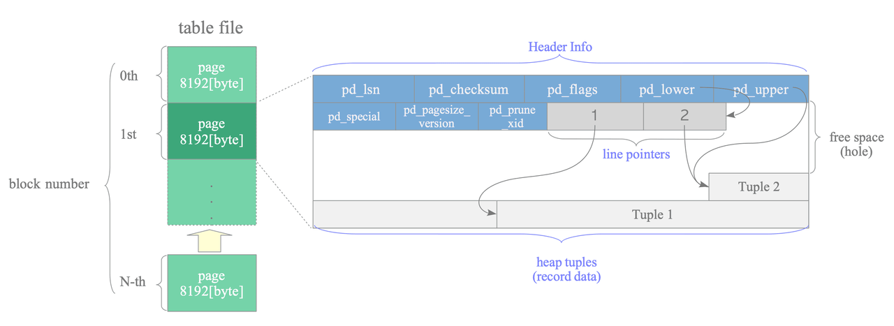
A page within a table contains three kinds of data:
- heap tuple(s) – A heap tuple is a record data itself. Heap tuples are stacked in order from the bottom of the page.
- line pointer(s) – A line pointer is a pointer to each heap tuple. Line pointers form a simple array that plays the role of an index to the tuples. When a tuple is added to the page, a new line pointer is pushed onto the array to point to the new tuple.
- header data – A header data (struct
PageHeaderData) is allocated in the beginning of the page. It contains information about the page.
The PageHeaderData is defined like this:
typedef struct PageHeaderData
{
 /* XXX LSN is member of *any* block, not only page-organized ones */
 PageXLogRecPtr pd_lsn;  /* LSN: next byte after last byte of xlog
         * record for last change to this page */
 uint16  pd_checksum; /* checksum */
 uint16  pd_flags;  /* flag bits, see below */
 LocationIndex pd_lower;  /* offset to start of free space */
 LocationIndex pd_upper;  /* offset to end of free space */
 LocationIndex pd_special; /* offset to start of special space */
 uint16  pd_pagesize_version;
 TransactionId pd_prune_xid; /* oldest prunable XID, or zero if none */
 ItemIdData pd_linp[FLEXIBLE_ARRAY_MEMBER]; /* line pointer array */
} PageHeaderData;

typedef PageHeaderData *PageHeader;

typedef uint64 XLogRecPtr;
For now the most important are:
pd_checksum- checksum of the pagepd_lower,pd_upper- points to the end/start of the free heap spacepd_special– This variable is for indexes. In the page within tables, it points to the end of the page. (In the page within indexes, it points to the beginning of special space, which is the data area held only by indexes and contains the particular data according to the kind of index types such as B-tree, GiST, GiN, etc.)
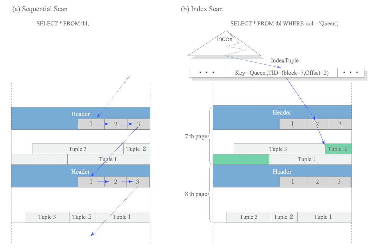
To identify a tuple within the table, a tuple identifier (TID) is used internally. A TID comprises a pair of values: the block number of the page that contains the tuple, and the offset number of the line pointer that points to the tuple.
Reading Heap Tuples
Two typical access methods, sequential scan and B-tree index scan, are outlined here:
- Sequential scan – It reads all tuples in all pages sequentially by scanning all line pointers in each page.
- B-tree index scan – It reads an index file that contains index tuples. If the index tuple with the key that you are looking for has been found, PostgreSQL reads the desired heap tuple using the obtained TID value.
PostgreSQL has a component called planner (or query optimizer) that takes a parsed SQL query and figures out the most efficient way to execute it.
The costs of sequential scans and index scans are estimated by cost_seqscan() and cost_index() respectively.
The seq_page_cost vs random_page_cost ratio is the key lever. The default values of seq_page_cost and random_page_cost are 1.0 and 4.0 respectively which means PostgreSQL assumes random access is four times slower than sequential. This default is based on HDDs. When using SSDs, random_page_cost should be lowered to around 1.0, otherwise the planner may select ineffective plans.
Sequential scan is typically chosen for cases when the table being scanned is small or the percentage of rows returned outweighs using an index. If a query returns ~10% of rows, a sequential scan is probably faster.
Bitmap scans act as a middle ground. If an index scan or a sequential scan aren't the perfect option, Postgres can use a bitmap index scan as a hybrid approach. It is typically chosen when a query matches too many rows for a regular index scan, but not so many that a sequential scan would be the best option.
It works in two phases: first builds an in-memory bitmap of matching pages from the index, then fetches only those pages from the heap; this provides better random I/O behaviour than a pure index scan.
Index-Only Scans and Visibility Maps
PostgreSQL uses a performance optimization called Index-Only Scan that avoids accessing heap pages when possible. The challenge is that index tuples lack transaction metadata (t_xmin, t_xmax), which is needed for visibility checks in concurrent transactions.
The solution is the Visibility Map (VM): when a heap page is marked as fully visible in the VM, all tuples on that page are known to be visible to all transactions. For these pages, PostgreSQL can retrieve all necessary data directly from the index without accessing the heap at all.
For pages with uncertain visibility, heap access is still required to verify which tuple versions are visible to the current transaction.
This optimization significantly reduces I/O costs for queries that can be satisfied by index data alone, especially for large tables where heap pages may be scattered across disk.
Writing Heap Tuples
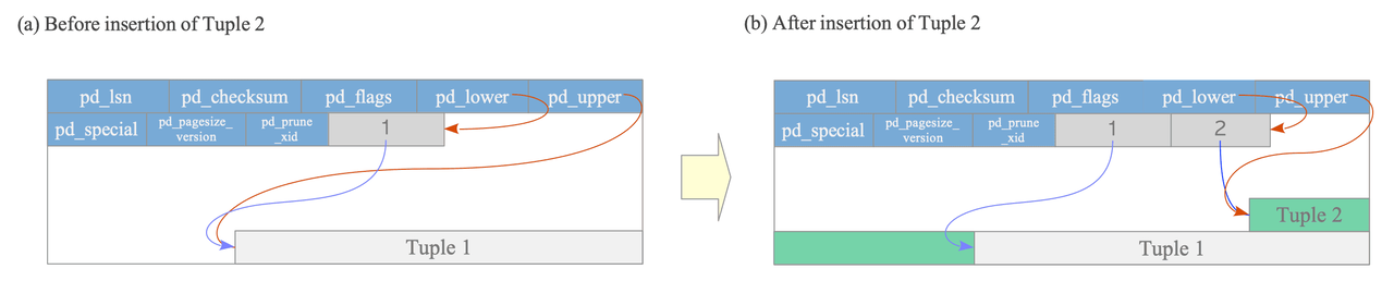
To understand how PostgreSQL writes tuples into a page, let's consider a simple table with a single page that initially holds one tuple.
At that point, pd_lower points to the first line pointer, and that line pointer, along with pd_upper, both reference the same first tuple in the page.
When a second tuple is inserted, PostgreSQL places it right after the first one and appends a new line pointer to the array.
The new line pointer references the newly written tuple, while pd_lower advances to point at this second line pointer and pd_upper shifts down to point at the second tuple.
Along with these pointer updates, other metadata fields in the page header are also updated accordingly.
Heap Only Tuple Optimization
The Heap Only Tuple (HOT) mechanism is an optimization that kicks in when an updated row can be stored on the same page as its predecessor. It conserves space in both index and table pages, and reduces the amount of work VACUUM needs to do.
Consider a table "tbl" with columns id (primary key) and data. The table has 1,000 rows; the last one (id = 1000) lives on page 5 of the table heap, referenced by an index entry pointing to position (5, 1). When you run:
UPDATE tbl SET data = 'B' WHERE id = 1000;Without HOT, PostgreSQL writes a new tuple to the heap and a new entry into the index page. Every update therefore bloats the index, and cleaning up those stale index entries is expensive, both in write cost and in VACUUM overhead.
HOT avoids the extra index write under two conditions:
- The new tuple fits on the same page as the old one. If the row migrates to a different page, a new index entry must be written.
- The indexed column(s) are not modified. If the update changes a value that is part of an index key, a new index entry is required regardless of page placement.
When these conditions are met, PostgreSQL skips inserting a new index tuple.
Instead, it marks the old tuple with the HEAP_HOT_UPDATED flag and the new tuple with the HEAP_ONLY_TUPLE flag. The existing index entry continues to point to the old tuple's line pointer, no index page is touched.
Reading a HOT-updated row via index scan then works like this:
- Follow the index entry to line pointer [1].
- Read the old tuple (Tuple_1), which is flagged
HEAP_HOT_UPDATED. - Follow Tuple_1's
t_ctidto reach the new tuple (Tuple_2). - Apply the visibility rules to decide which version is the one to return.
A problem arises once Tuple_1 becomes dead and gets removed: the index still points to its line pointer, but the tuple is gone, making Tuple_2 unreachable.
PostgreSQL solves this through pruning: before Tuple_1 is physically removed, its line pointer is redirected to point at Tuple_2's line pointer. The index entry therefore still leads to the correct live tuple through an extra indirection hop, without any change to the index itself.
Pruning can happen opportunistically during any SQL command whenever PostgreSQL judges it appropriate.
Alongside pruning, PostgreSQL also performs defragmentation: it reclaims the space occupied by dead HOT tuples on the page. Crucially, this does not touch the index at all, so it is significantly cheaper than a full VACUUM pass.
Complete description can be found here.
Process and Memory Architecture
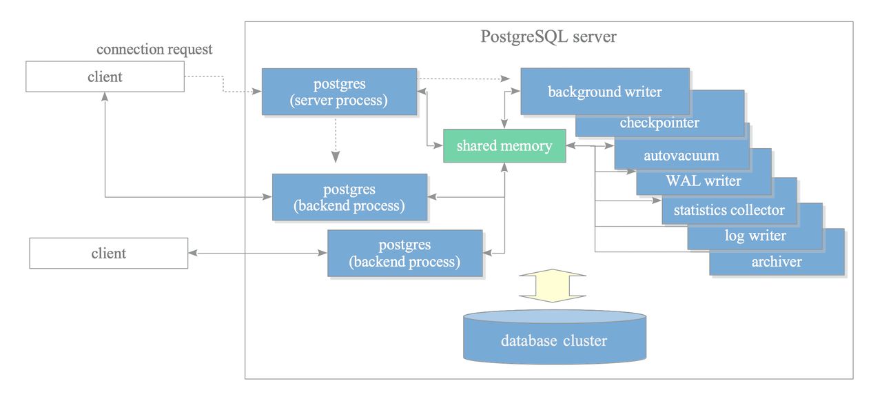
A collection of multiple processes that cooperatively manage a database cluster is usually referred to as a ‘PostgreSQL server’. It contains the following types of processes:
-
Postgres server process: is the parent of all processes within a PostgreSQL server. It allocates a shared memory area, initiates various background processes, starts replication-related processes and background worker processes as needed, and waits for connection requests from clients (by listening on port 5432). When a connection request is received, it spawns a backend process to handle the client session.
-
Backend process: handles all queries issued by one connected client. It communicates with the client using a single TCP connection and terminates when the client disconnects. PostgreSQL supports concurrent connections from multiple clients, with the maximum number controlled by the
max_connectionsparameter (default: 100).If clients frequently connect and disconnect from a PostgreSQL server, it can increase the cost of establishing connections and creating backend processes. To deal with such a case, a connection pooling middleware such as pgbouncer can be used.
-
Background processes:
- Background writer: writes dirty pages on the shared buffer pool to a persistent storage.
- Checkpointer: this process performs the checkpoint process.
- Autovacuum launcher: it requests the postgres server to create the autovacuum workers.
- WAL writer: writes and flushes the WAL data on the WAL buffer to persistent storage periodically.
- IO worker: handle read operations asynchronously, offloading I/O tasks from regular backend processes.
- Others: WAL summarizer, statistics collector, archiver and logging collector.
-
Replication-associated processes
Memory architecture in PostgreSQL can be classified into three broad categories:
- Local memory area
- Dynamic Shared Memory
- Shared memory area
Each backend process allocates a local memory area for query processing. The three major areas are:
work_mem: used by the executor for sorting, distinct and joining operations.maintenance_work_mem: various maintenance operations like VACUUM use this mem area.temp_buffers: executor uses this area for storing temporary tables.
Dynamic Shared Memory it's an on-demand mem space used by parallel query for inter-process communications between postgres processes.
The shared memory area is allocated at startup. There are three major areas:
- Shared buffer pool: tables and indexes pages are loaded from persistent storage here to be operated on directly
- WAL buffer: is a buffering are where WAL data is stored before writing it to persistent storage
- Commit log (CLOG): keeps the state of all transactions (in_progress,committed, aborted) for the concurrency control mechanism.
Query Processing
Although the parallel query implemented in version 9.6 uses multiple background worker processes, a backend process basically handles all queries issued by the connected client. This backend consists of five subsystems:
- Parser
- Analyzer
- Rewriter
- Planner
- Executor
SQL Statement
↓
┌─────────────────────────────────┐
│ Backend Process │
│ │
│ ┌──────────────────────────┐ │
│ │ Parser │ │
│ └──────────┬───────────────┘ │
│ │ (parse tree) │
│ ↓ │
│ ┌──────────────────────────┐ │
│ │ Analyzer/Analyser │ │
│ └──────────┬───────────────┘ │
│ │ (query tree) │
│ ↓ │
│ ┌──────────────────────────┐ │
│ │ Rewriter │ │
│ └──────────┬───────────────┘ │
│ │ (query tree) │
│ ↓ │
│ ┌──────────────────────────┐ │
│ │ Planner │ │
│ └──────────┬───────────────┘ │
│ │ (plan tree) │
│ ↓ │
│ ┌──────────────────────────┐ │
│ │ Executor │ │
│ └──────────┬───────────────┘ │
│ │ │
└─────────────┼───────────────────┘
↓
Result
↓
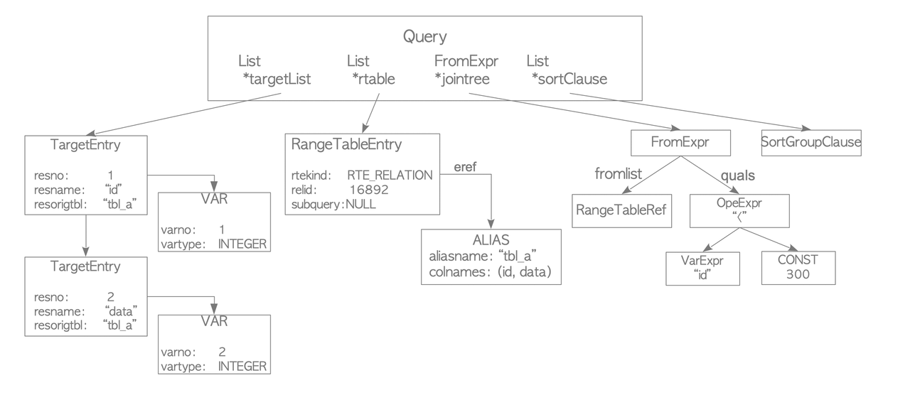
ClientThe parser generates a parse tree from sql plain text and only checks the syntax of an input when generating a parse tree. Therefore, it only returns an error if there is a syntax error in the query. For example:
testdb=# SELECT id, data FROM tbl_a WHERE id < 300 ORDER BY data;becomes:
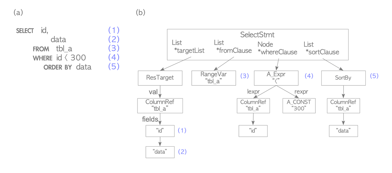
The analyzer runs a semantic analysis of the parse tree and generates a query tree. The root is the Query structure containing the command type, metadata, and leaves structured as lists or trees for each clause.
The Query structure has four key components. The targetlist contains the result columns, and if the input uses an asterisk, the analyzer expands it to all columns. The range table holds the relations and tables used in the query, including their OID and name. The join tree stores the FROM and WHERE clauses. Finally, the sort clause contains a list of SortGroupClause elements.
The rewriter is the system that realizes the rule system. It transforms a query tree according to the rules stored in the pg_rules system catalog, if necessary.
For example views in PostgreSQL are implemented by using the rule system.
The planner receives a query tree from the rewriter and generates a (query) plan tree that can be processed by the executor most effectively. Its objective is to do cost optimization.
When using the EXPLAIN command we are effectively showing the query plan tree.
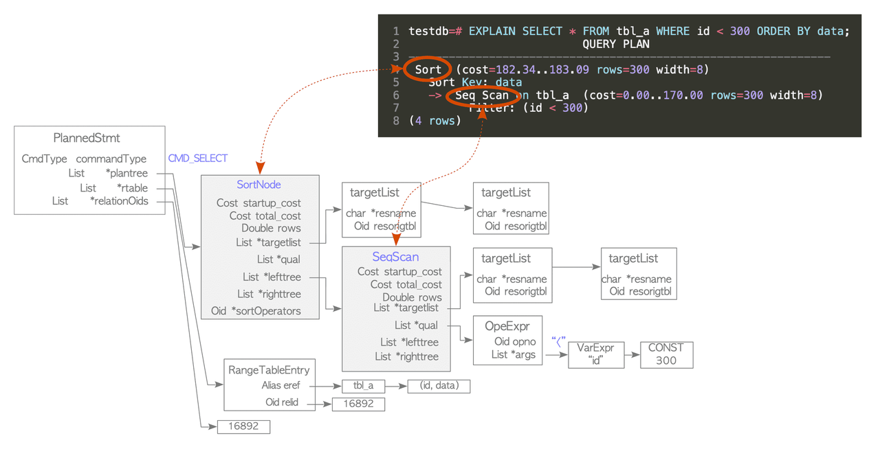
The plan tree is composed of nodes, those nodes contains information necessary by the executor for processing.
The executor operates on tables and indexes via the buffer manager. When processing a query, the executor uses some memory areas, such as temp_buffers and work_mem, allocated in advance and creates temporary files if necessary.
In the output of the explain node each line is a plan node. The tree is read bottom-up, the executor starts at the deepest indented node and works toward the root:
Seq Scanruns first → scans the heap, appliesid < 300filterSortruns second → takes those rows and sorts bydata
The cost number are divided in the following way:
- The startup cost is the cost before the first heap tuple is fetched. For Seq Scan it's 0.00 because it can start emitting tuples immediately. Instead, for an index scan, it must traverse the B-tree before. Only after reaching the leaf node it will emit the first TID.
- The run cost depends on the type of node and is calculated by a sum of various constants (cpu cost, i/o cost per page and others).
- The total cost is the sum of the costs of both start-up and run costs.
- The rows is the estimated number of rows this node will return. Comes from
pg_statistic/ANALYZE. - The width is the average size of one row in bytes. Used to estimate memory consumption.
These costs are in arbitrary dimensionless units, they only matter relative to each other. seq_page_cost = 1.0 is the baseline everything else is measured against.
(cost=182.34..183.09 rows=300 width=8)
  └──┬──┘  └───┬───┘  └──┬──┘  └─┬─┘
  startup    total    estimated  avg row
   cost      cost      rows     size (bytes)
Plain EXPLAIN only shows estimates; EXPLAIN ANALYZE actually executes the query and shows real numbers alongside:
EXPLAIN ANALYZE SELECT * FROM tbl_a WHERE id < 300 ORDER BY data;

 Sort  (cost=182.34..183.09 rows=300 width=8)
       (actual time=4.200..4.350 rows=287 loops=1)
   Sort Key: data
   Sort Method: quicksort  Memory: 36kB
   ->  Seq Scan on tbl_a  (cost=0.00..170.00 rows=300 width=8)
                           (actual time=0.021..1.812 rows=287 loops=1)
         Filter: (id < 300)
         Rows Removed by Filter: 713
 Planning Time: 0.5 ms
 Execution Time: 4.6 ms
actual time measures pure executor time inside the node in milliseconds, not considering the time spent converting output or transmission to the client.
The new fields are:
- loops: how many times this node was executed. Important for joins, an inner node in a nested loop runs once per outer row.
- sort method: tells you which sort alg. was applied and the quantity of memory used. If it says external
merge Disk: Xkb, the sort spilled to disk because work_mem was too small.
Finally we have EXPLAIN (ANALYZE, BUFFERS) which also show I/O stats.
EXPLAIN (ANALYZE, BUFFERS) SELECT * FROM tbl_a WHERE id < 300 ORDER BY data;

 Sort  (cost=182.34..183.09 rows=300 width=8)
       (actual time=4.200..4.350 rows=287 loops=1)
   Buffers: shared hit=48
   ->  Seq Scan on tbl_a ...
         Buffers: shared hit=45 read=5
The new important fields are:
- shared hit: number of pages served from the buffer manager (shared memory) so no disk I/O.
- read: number of pages fetched from disk (or OS cache) via
pread(), the expensive path. - written: number of dirty pages written back to disk during query execution.
For a complete explanation of formulas, math and the limitations behind cost estimation see: Cost Estimation in Single-Table Query
Planner Processing in detail
The planner performs three steps:
- Carry out preprocessing: some examples are: simplifying target lists, limit clauses, eval constant expressions, flattening and/or expressions.
- Get the cheapest access path by estimating the costs of all possible access paths
- Create the plan tree from the cheapest path.
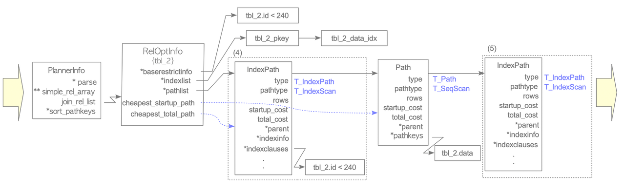
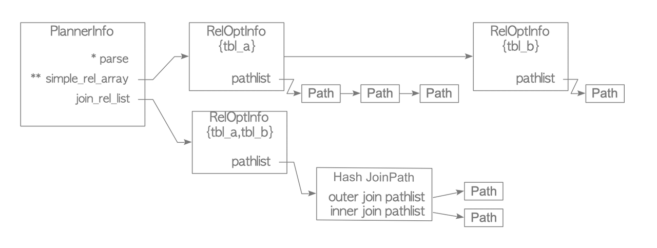
To plan the cheapest access path, the planner creates a RelOptInfo structure which contains the access paths and their corresponding costs.
The structure is stored in the simple_rel_array of the PlannerInfo structure.
In its initial state, the RelOptInfo holds the baserestrictinfo and the indexlist if related indexes exist. The baserestrictinfo stores the WHERE clauses of the query, and the indexlist stores the related indexes of the target table.
After the initialization of the RelOptInfo struct the planner estimates the costs of all possible access paths, and add them to the struct.
Details of this processing:
- A path is created, the cost of the sequential scan is estimated, and the estimated costs are written to the path. Then, the path is added to the
pathlistof theRelOptInfostructure. - If indexes related to the target table exist, index access paths are created, all index scan costs are estimated, and the estimated costs are written to the path. Then, the index paths are added to the
pathlist. - If the bitmap scan can be done, bitmap scan paths are created, all bitmap scan costs are estimated, and the estimated costs are written to the path. Then, the bitmap scan paths are added to the
pathlist.
After that, the planner gets the cheapest access path in the pathlist of the structure and estimates limit, order_by if necessary.
Here is an example from InterDB.
Given this table:
testdb=# \d tbl_2
     Table "public.tbl_2"
 Column |  Type   | Modifiers
--------+---------+-----------
 id     | integer | not null
 data   | integer |
Indexes:
    "tbl_2_pkey" PRIMARY KEY, btree (id)
    "tbl_2_data_idx" btree (data)

testdb=# SELECT * FROM tbl_2 WHERE id < 240;
The steps are:
- Create a
RelOptInfostruct - Add the WHERE clause to the
baserestrictinfo, and add the indexes of the target table to theindexlist. In this example, a WHERE clauseid<240is added to thebaserestrictinfo, and two indexes,tbl_2_pkeyandtbl_2_data_idx, are added to theindexlist. - Estimate the cost of the sequential scan, and add the path to the
pathlistof theRelOptInfo. - Estimate the cost of the index scans and add them to the
pathlist. Note that when adding access path they're inserted in sort order of the total cost. - Create a new
RelOptInfostructure with the cheapest path.
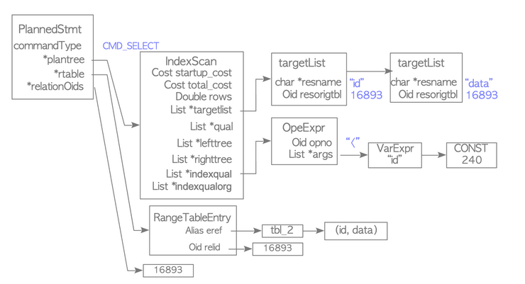
After that the planner generates a plan tree from the cheapest path.
The plan tree is composed of different nodes like:
PlannedStmt which is the root of the tree and contains information such as:
- commandType: stores type of operation, such as SELECT and UPDATE.
- rtable: stores range table entries.
- relationOids: stores oids of the related tables.
- plantree: stores a plan tree that is composed of plan nodes.
The plan trees is composed of various plan nodes.
The PlanNode structure is the base node and other nodes (SeqScanNode,IndexScanNode) always contain it. A PlanNode contains fields such as:
- start-up cost and total_cost.
- rows is the number of rows to be scanned, which is estimated by the planner.
targetliststores the target list items contained in the query tree.- qual is a list that stores qual conditions.
- lefttree and righttree are the nodes for adding the children nodes.
Before we described the process for creating a plan tree of a single-table query, in the following is described the same process for multiple-table queries.
The preprocessing phase is similar, there are only some added operations like converting subqueries to join if possible and transforming outer joins to inner joins if possible.
Then based on the number of tables in the query and based on the parameter geqo_threshold (default 12) one of the two method is applied:
if n_tables > geqo_thresholdthen a genetic algorithm is used. The problem is in fact subjected to combinatorial explosion and for this reason a fast but sub-optimal solution is choosed instead of a optimal but slow solution.- otherwise a dynamic programming algorithm is used.
The pseudocode for the dynamic programming algorithm is the following:
function find_cheapest_plan(tables[1..n]):

    # Step 1: solve all singles
    for each table T:
        best_plan({T}) = cheapest way to read T

    # Steps 2..n: solve increasingly larger groups
    for size = 2 to n:
        for each subset S of tables where |S| = size:

            best = infinity

            # try every way to split S into two non-empty groups
            # where left_size <= right_size (to avoid duplicates)
            for left_size = 1 to size / 2:
                for each subset L of S where |L| = left_size:
                    R = S - L

                    # skip duplicate: when both halves are same size,
                    # only consider L < R to avoid trying the same split twice
                    if left_size = size - left_size and L > R:
                        skip

                    # both L and R were solved in earlier steps
                    left_plan  = best_plan(L)
                    right_plan = best_plan(R)

                    # try every join method in both directions
                    for each method in [nested_loop, merge_join, hash_join]:
                        cost1 = estimate(method, outer=left_plan,  inner=right_plan)
                        cost2 = estimate(method, outer=right_plan, inner=left_plan)
                        best = min(best, cost1, cost2)

            best_plan(S) = best

    # the answer is the best plan for the full set
    return best_plan(tables[1..n])
Given n tables {T₁, T₂, ..., Tₙ}, build solutions bottom-up by group size k:
- k = 1: For each table Tᵢ, find its cheapest access path (sequential scan, index scan, etc.). Store it as best_plan({Tᵢ}).
- k = 2: For each pair {Tᵢ, Tⱼ}, the only split is {Tᵢ} + {Tⱼ}. Try all join methods in both directions. Store the cheapest as best_plan({Tᵢ, Tⱼ}).
- k = 3: For each triple, try all 1+2 splits. Example: {A,B,C} → A+{B,C}, B+{A,C}, C+{A,B}. Both sides already solved. Keep the cheapest.
- k = 4: Now two kinds of splits appear: 1+3 and 2+2. Example: {A,B,C,D} → A+{B,C,D}, ..., D+{A,B,C}, {A,B}+{C,D}, {A,C}+{B,D}, {A,D}+{B,C}. All sub-groups already solved.
- k = 5..n: Same pattern. Split sizes grow: 1+(k-1), 2+(k-2), ..., up to ⌊k/2⌋+(k-⌊k/2⌋). Every sub-group was solved at a smaller k.
- k = n: One group remains — all tables. The cheapest plan found for it is the final answer.
The key properties of this algorithm are:
- Every sub-problem is solved exactly once and reused many times.
- All join methods and directions are tried at every split.
- Total sub-problems = 2ⁿ, which explodes past n ≈ 12, hence PostgreSQL's switch to a genetic algorithm.
This algorithm is known in the literature as DPsize (Dynamic Programming by size), originally introduced by Selinger et al. It produces bushy join trees, meaning it considers not only left-deep plans (where one new table is added at each step) but also plans where two independently computed sub-joins are combined (e.g., (A ⋈ B) ⋈ (C ⋈ D)).
Bushy trees can be significantly cheaper than left-deep trees in certain scenarios like when small tables can be paired together independently, keeping intermediate results small throughout.
Join Operations
PostgreSQL supports three join operations:
- Nested loop join
- Merge join
- Hash join
The nested loop join and the merge join in PostgreSQL have several variations.
Nested Loop Join scans the inner table once for every row in the outer table, checking the join condition each time. It's simple and works with any join condition, but can be slow for large tables. The start-up cost is 0 while the run cost is defined primarily by the product of the sizes of the outer and inner tables.
The cost of this join is always estimated, but this join operation is rarely used because more efficient variations are usually used.
PostgreSQL has a variation called materialized nested loop join which reduces the total scanning cost of the inner table.
Before running a nested loop join, the executor writes the inner table tuples to work_mem or a temporary file by scanning the inner table once.
This has the potential to process the inner table tuples more efficiently than using the buffer manager, especially if at least all the tuples are written to work_mem.
There's another variation called indexed nested loop join which uses the index on the inner table to look up the tuples satisfying the join condition for each tuple of the outer table.
Unlike the nested loop join, the merge join can only be used in natural joins and equi-joins.
The basic merge join sorts both tables on the join key, then walks through them in parallel to find matches.
The startup cost comes from sorting both sides, O(N log N) each, while the actual merging is only O(N_outer + N_inner). It only works for equi-joins.
When the inner table benefits from being cached for efficient rescanning, PostgreSQL adds a Materialize node on top of the sorted inner result, producing a materialized merge join.
If the outer table already has an index on the join key, PostgreSQL can skip sorting it entirely and use an index scan instead, while still sorting (or materializing) the inner table. In the best case, when both tables have suitable indexes, PostgreSQL uses index scans on both sides, eliminating sorting costs altogether; this is the indexed merge join and typically the cheapest variant.
Similar to the merge join, the hash join can be only used in natural joins and equi-joins.
The behavior changes depending on whether the inner table fits in memory.
When the inner table is small enough (25% or less of work_mem), PostgreSQL uses a simple in-memory hash join.
It works in two phases:
- The "build" phase scans the entire inner table and inserts every tuple into a hash table (called a "batch") organized into buckets whose count is always a power of 2.
- The "probe" phase scans the outer table, hashes each tuple's join key, looks up the matching bucket, and joins any tuples that satisfy the condition. The overall cost is roughly O(N_outer + N_inner).
When the inner table is too large for a single in-memory batch, PostgreSQL switches to a hybrid hash join with skew.
It creates multiple batches, one in memory and the rest as temporary files on disk. Each tuple is routed to a batch based on a portion of its hash key bits.
The build and probe phases then repeat for each batch in successive rounds.
The first round processes the in-memory batch directly, while later rounds require reading and writing temp files, which is more expensive. To mitigate this, PostgreSQL adds a special "skew" batch that holds inner tuples expected to match the most common values (MCVs) of the outer table's join attribute. This way, if the data distribution is skewed, say 10% of customers account for 70% of purchases, most outer tuples get processed in the cheap first round via the skew batch, avoiding costly disk I/O in later rounds.
Finally, the hash join can also incorporate index scans. During the probe phase, if the outer table has a usable index for a WHERE clause filter, PostgreSQL will use an index scan instead of a sequential scan to feed tuples into the probe side.
Parallel Query
Parallel Query is a feature that processes a single query using multiple processes (Workers).
The PostgreSQL process that executes the query becomes the Leader and starts up multiple Worker processes. Each Worker process then performs scan processing, and returns the results sequentially to the Leader process. The Leader process aggregates the results.
The configuration parameter parallel_leader_participation, allows the Leader process to also process queries while waiting for responses from Workers. The default is on.
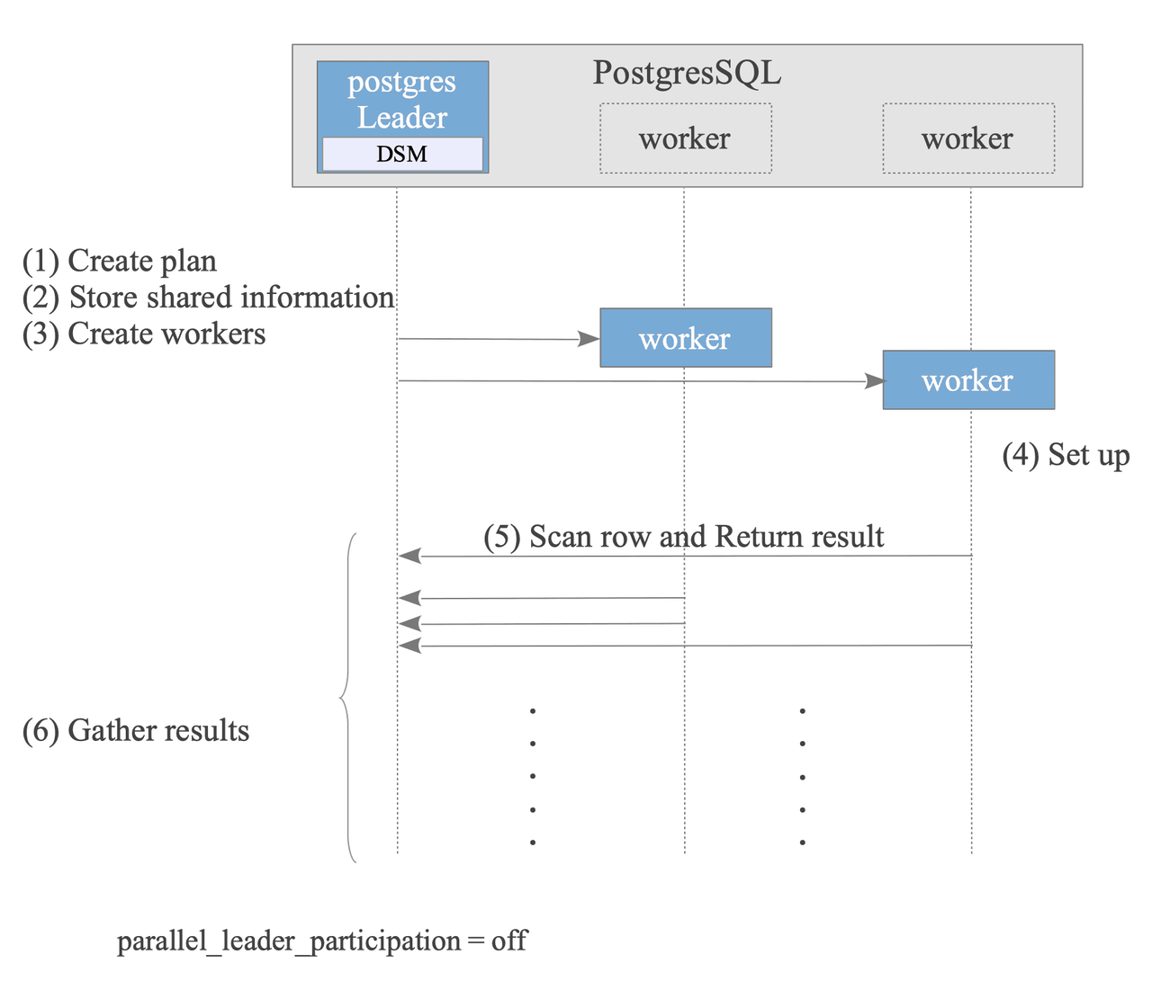
- Leader Creates Plan: The optimizer creates a plan that can be executed in parallel. It's done by adding the following nodes to the plan:
GatherNode,GatherMerge,AppendandAppendMerge,Finalize/Partial Aggregate. The nodes executed by Workers are generally the subplan tree below those nodes, and the parallel_safe value is set to True. - Leader Stores Shared information: To execute the plan on both the Leader and Worker nodes, the Leader stores necessary information in its Dynamic Shared Memory (DSM) area.
- Leader Creates Workers.
- Worker Sets up State: Each worker reads the stored shared information to sets up its state, ensuring a consistent execution environment with the Leader.
- Worker Scans rows and returns results.
- Leader Gathers results.
- After the query finishes, the Workers are terminated, and the Leader releases the DSM area.
Concurrency Control
Above Read Committed, PostgreSQL offers two stronger isolation modes:
- Snapshot Isolation (Repeatable Read)
- Serializable Snapshot Isolation (Serializable).
In particular it uses MVCC for SI and Optimistic Concurrency control for DML (Data manipulation Language, e.g. SELECT, UPDATE, INSERT, DELETE) while it uses two-phase locking (2PL) for DDL (Data Definition Language, e.g. CREATE TABLE, etc).
At the start of a transaction, the transaction manager assigns a unique identifier known as a transaction ID (txid). There are three special txid:
0meansInvalid.1meansBootstrap, which is used in the initialization of the db cluster.2meansFrozen, which is a mechanism used to handle the integer overflow of the transaction id.
Txids can be compared with each other to understand the "time position" of the transaction and therefore the visibility of the other transactions for the current one.
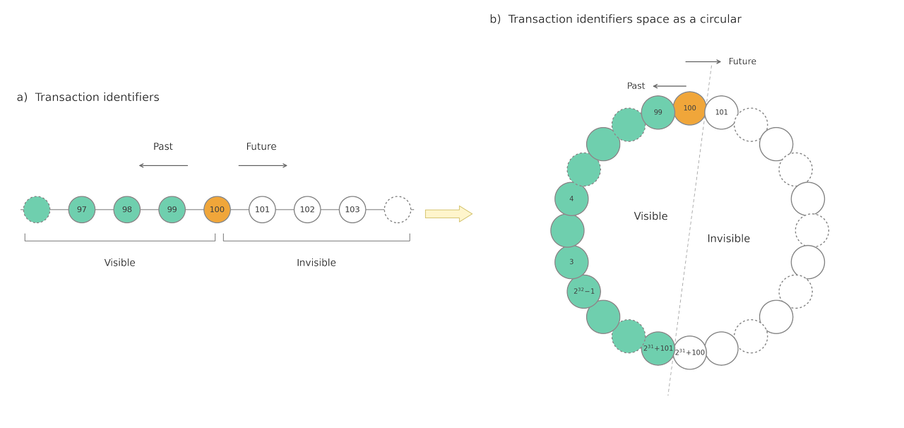
Since the txid space is insufficient in practical systems, PostgreSQL treats the txid space as a circle.
Heap tuples in table pages are of two types: usual data tuples and TOAST tuples.
In the usual data tuples, the HeapTupleHeaderData structure contains different info:
- t_xmin holds the txid of the transaction that inserted this tuple.
- t_xmax holds the txid of the transaction that deleted or updated this tuple. If this tuple has not been deleted or updated,
t_xmaxis set to 0, which means INVALID as seen before. - t_cid stores the command id (cid): a zero-based counter of how many SQL commands have already run in the current transaction before the one that produced this tuple. In BEGIN; INSERT; INSERT; INSERT; COMMIT;, the three inserted tuples get
t_cidvalues of 0, 1, and 2 respectively. - t_ctid holds a tid that locates a tuple within the table. If the tuple has been updated, its
t_ctidpoints to the new version; otherwise it points to itself.
PostgreSQL does not overwrite data in place by using "slotted page" as heap page: line pointers grow downward from the header, and tuple data stacks upward from the bottom, with free space in between. Each tuple carries MVCC metadata described before where t_ctid act as pointer to the next version of the same row, or to itself if it's the latest.
When multiple transactions insert rows, each new tuple simply gets appended on top of the latest tuple and a new line pointer is allocated at the top. The tuples from different transactions coexist in the same page, visibility is determined later by checking each tuple's t_xmin/t_xmax against the reader's snapshot, not by physical separation.
When a row is updated, PostgreSQL logically deletes the old tuple (writing the updating transaction's ID into t_xmax) and inserts a brand-new tuple with the new data.
The old tuple's t_ctid is rewritten to point to the new one, forming a version chain. This is why updates cause table bloat, every update leaves a dead tuple behind.
When a row is deleted, only t_xmax is set. The tuple remains physically in the page as a dead tuple until VACUUM reclaims the space, resetting those line pointers to "unused" and freeing the bytes for future inserts. The Free Space Map (FSM) then knows this page has room again.
Commit Log (CLOG)
PostgreSQL holds the statuses of transactions in the Commit Log (CLOG). It's allocated to shared memory and is used throughout transaction processing.
There are four transaction states: IN_PROGRESS, COMMITTED, ABORTED, and SUB_COMMITTED.
The clog comprises one or more 8 KB pages in shared memory. It logically forms an array, where the indices of the array correspond to the respective transaction ids, and each item in the array holds the status of the corresponding transaction id.
When PostgreSQL shuts down or whenever the checkpoint process runs, the data of the clog are written into files stored in the pg_xact subdirectory. (Note that pg_xact was called pg_clog in versions 9.6 or earlier.) These files are named ‘0000’, ‘0001’, and so on.
PostgreSQL flushes its transaction status data (the 'clog') to the pg_xact folder whenever a checkpoint occurs or the system shuts down.
New pages are appended to the clog as it fills, causing it to expand over time. However, to keep the system efficient, the Vacuum process regularly prunes unnecessary old data from these pages and files.
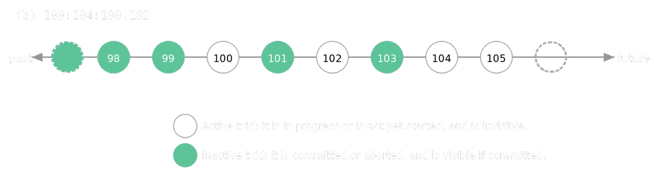
Transaction Snapshot
A snapshot is a data set that records which transactions are active (either in progress or not yet started) at a specific moment. PostgreSQL uses this to determine which versions of data (tuples) a transaction is allowed to see.
PostgreSQL represents snapshots using three main components:
- xmin: The earliest transaction ID (txid) that is still active. All transactions with a lower ID are already committed or aborted.
- xmax: Any transaction with this ID or higher is considered "not yet started" and is invisible.
- xip_list: A list of specific active txids that fall between xmin and xmax.
The timing of when a snapshot is taken depends on the transaction's isolation level:
- SI: A new snapshot is obtained at the start of every SQL command. This allows the transaction to see changes committed by others between commands.
- SSI: A single snapshot is obtained when the first SQL command is executed and is reused for the entire transaction. This ensures the data stays consistent throughout the session.
SSI Implementation
Conceptually, there are three types of conflicts: wr-conflicts (Dirty Reads), ww-conflicts (Lost Updates), and rw-conflicts.
However, wr- and ww-conflicts do not need to be considered because PostgreSQL prevents such conflicts, as shown in the previous sections. Thus, SSI implementation in PostgreSQL only needs to consider rw-conflicts.
PostgreSQL takes the following strategy for the SSI implementation:
- Record all objects (tuples, pages, relations) accessed by transactions as SIREAD locks.
- Detect rw-conflicts using SIREAD locks whenever any heap or index tuple is written.
- Abort the transaction if a serialization anomaly is detected by checking detected rw-conflicts.
A SIREAD Lock is a Predicate Lock which is a pair of an object and (virtual) txids stored in shared memory that record which transaction has read which object. They exist at the tuple, page, and relation levels.
To save memory, PostgreSQL automatically aggregates granular locks: multiple tuple locks "promote" to a single page lock, and multiple page locks promote to a relation lock. However, a sequential scan is an exception, it immediately applies a relation-level lock, ignoring any specific WHERE clauses or available indexes.
An rw-conflict tracks the relationship between a transaction that reads data and a transaction that later writes to it. It consists of the SIREAD lock involved plus the two txids.
The system checks for these conflicts every time data is modified (via INSERT, UPDATE, or DELETE) using the CheckForSerializableConflictIn function. For instance, if Transaction A reads a row and Transaction B tries to update it, a conflict is recorded.
These records are evaluated during the execution and at the final COMMIT in pure Optimistic Concurrency control. If the system determines that these conflicts would break "serializability," it enforces a first-committer-win rule: only the first transaction to commit is allowed to finish; all others are rolled back.
Full details at Serializable Snapshot Isolation
Required Maintenance Process
The concurrency control mechanism requires the following:
- Remove dead tuples and corresponding index tuples.
- Remove unnecessary parts of the clog.
- Freeze old txids.
- Update FSM, VM, and the statistics.
PostgreSQL uses a 32-bit integer for transaction IDs, which means it can only track about 4.2 billion transactions. If a row is very old and the current txid "wraps around" past 2.1 billion, the old row suddenly looks like it was created in the "future", making it invisible to the system.
To dodge this bullet, the system employs Freeze Processing. During a vacuum, PostgreSQL identifies rows that have survived a specific number of transactions and marks them as "Frozen". By assigning these rows a special reserved status, either by setting their ID to a dedicated "always visible" value or by flipping a specific bit in the row header; this way the database ensures they stay permanently in the past.
This diligent bookkeeping allows the transaction counter to loop safely without the risk of losing access to your oldest data.
VACUUM Processing
Vacuum processing performs three main tasks:
- removing dead tuples (and the index entries pointing to them)
- freezing old transaction IDs to prevent txid wraparound
- updating housekeeping structures like the Free Space Map (FSM), Visibility Map (VM), and various statistics.
The process is organized into three main blocks plus a post-processing phase:
-
Scan Heap & Vacuum Indexes: PostgreSQL scans all pages of the target table, builds a list of dead tuples (stored in
maintenance_work_mem), freezes old txids where needed, and then removes index entries that point to those dead tuples. Ifmaintenance_work_memfills up before scanning is complete, it processes what it has and then resumes scanning.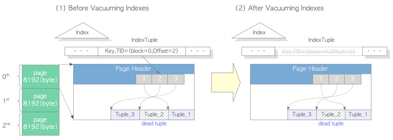
-
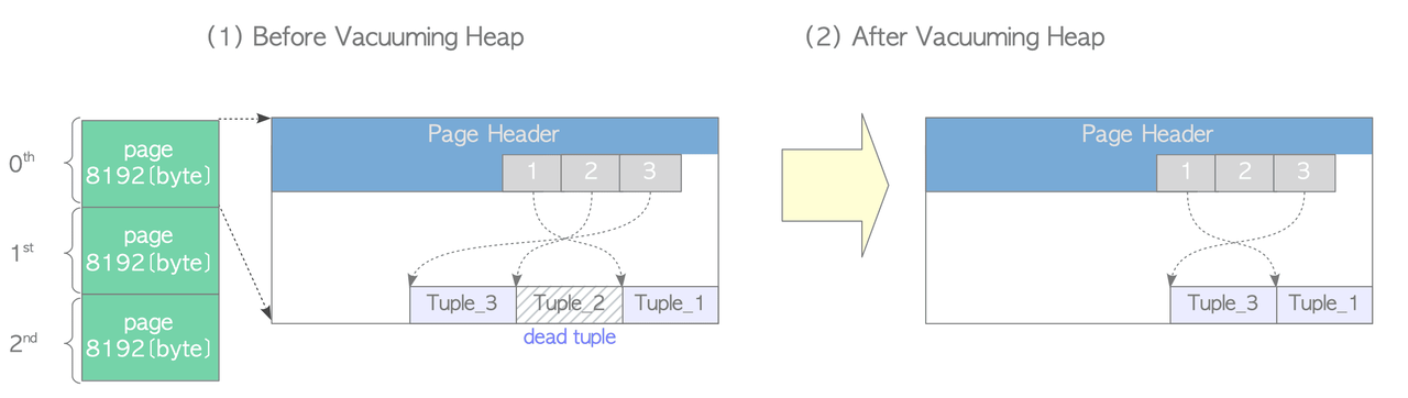
Vacuum Heap: Goes page by page, removing dead tuples and compacting live ones to eliminate fragmentation. FSM and VM are updated per page. Notably, empty line pointers are not removed, they're kept for reuse to avoid having to update all associated indexes.
-
Cleanup & Truncation: Runs
index_vacuum_cleanup()on indexes, updates per-table statistics and system catalogs, and truncates trailing empty pages from the table file to reclaim disk space. Only trailing empty pages can be removed this way; interior empty pages require VACUUM FULL.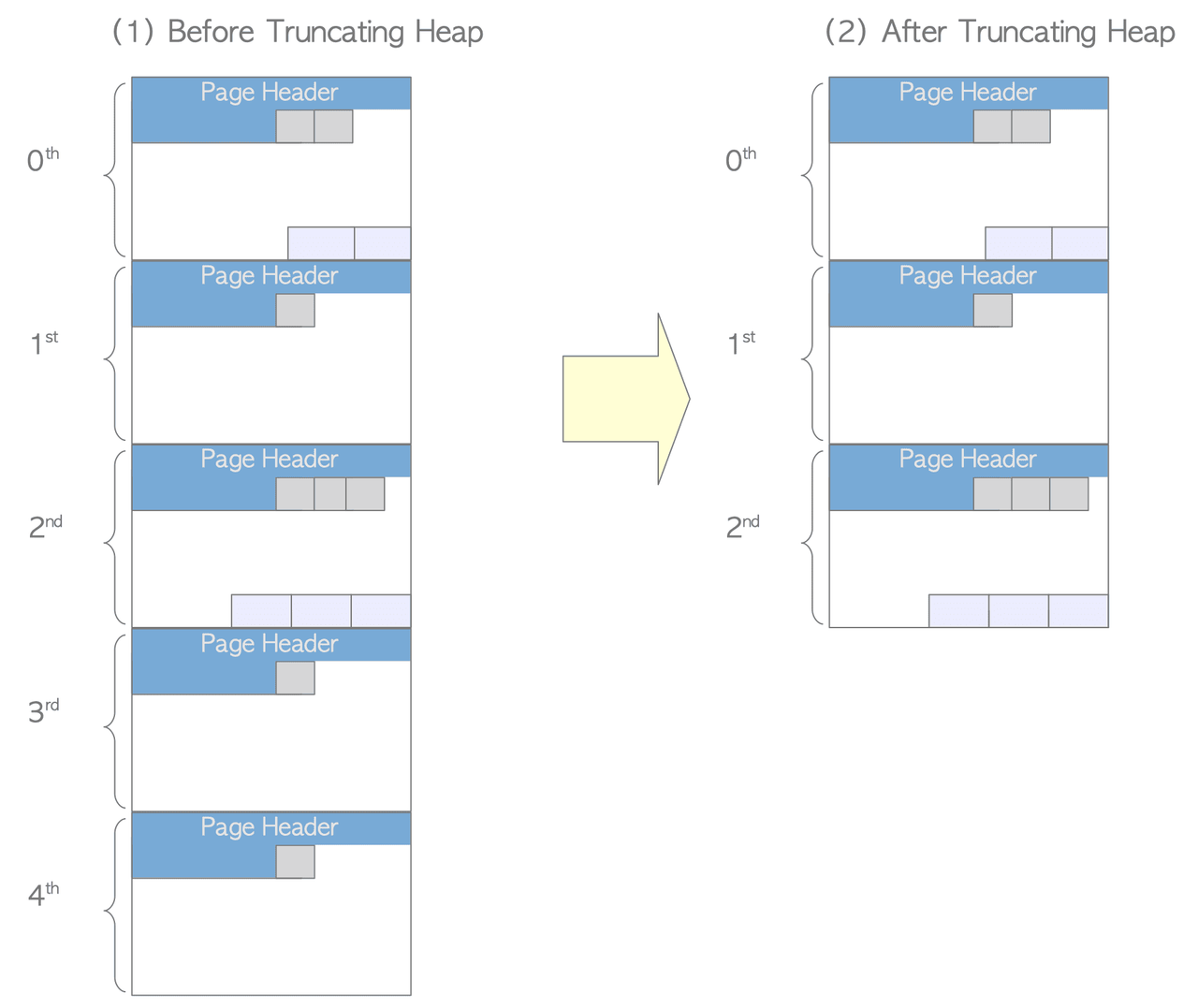
-
Post-processing: Updates global statistics and system catalogs, and removes now-unnecessary clog files.
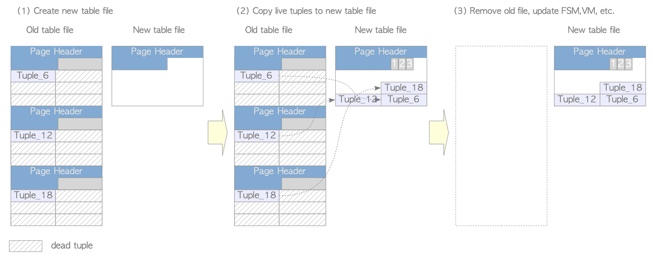
VACUUM FULL compacts table files by creating a new file, copying only live tuples to it, and removing the old file, addressing the limitation of concurrent VACUUM which removes dead tuples but doesn't reduce table size.
However, it requires exclusive access to the table during processing and temporarily uses up to twice the disk space, so it's used when the free space ratio in a table becomes excessive.
VACUUM processing is expensive. The Visibility Map (VM), reduces this cost by allowing VACUUM to skip pages that don't need processing.
Each table has its own VM file (stored with a _vm suffix, e.g. 18751_vm).
The VM tracks, per page, whether that page contains any dead tuples.
When VACUUM runs, it consults the VM and skips pages marked as clean, saving significant I/O.
Example: A table with 3 pages where pages 0 and 2 have dead tuples but page 1 does not; VACUUM will skip page 1 entirely based on the VM.
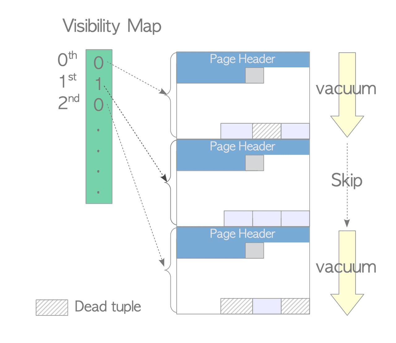
In PostgreSQL 9.6, the VM was extended to also record whether all tuples on a page are frozen. This second bit allows freeze processing (in eager mode) to skip already-frozen pages, further reducing unnecessary work.
Freeze processing prevents transaction ID (txid) wraparound, a fundamental PostgreSQL limit where txids eventually cycle back around and old tuples could be misidentified. Tuples with sufficiently old txids are "frozen" to avoid this. Processing runs in one of two modes depending on various conditions:
- Lazy mode (most often) which only scans pages that contain dead tuples by using the VM to skip clean pages. This mode has the limitation that it might leave some old tuples unfrozen.
- Eager mode which scans all pages regardless of dead tuples. With the VM improvement from PostgreSQL 9.6 described above now eager mode can scan only the relevant pages.
PostgreSQL attempts to remove old clog files whenever pg_database.datfrozenxid is updated (which happens at the end of eager-mode VACUUM).
The rule is: any clog file whose transactions are all older than the minimum pg_database.datfrozenxid across all databases in the cluster can be safely deleted, because every transaction in those files is already treated as frozen everywhere.
Buffer Manager
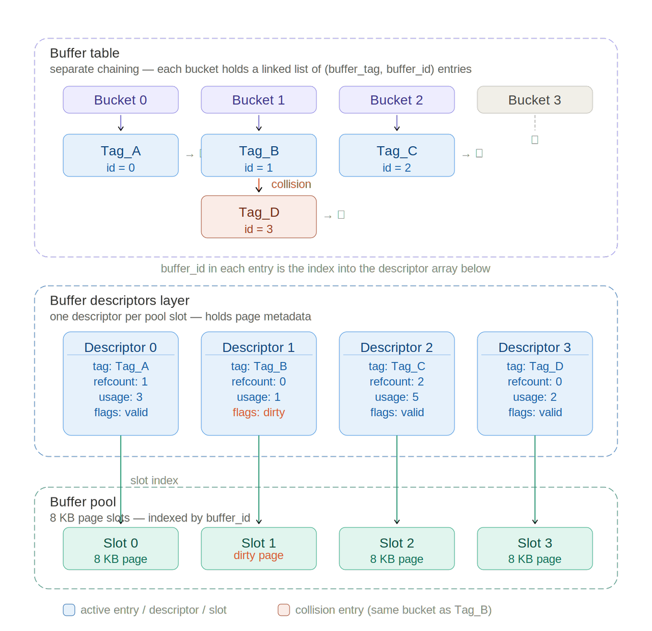
The buffer manager manages data transfers between shared memory and persistent storage, and it can have a significant impact on the performance of the DBMS. It is composed of three layers:
- Buffer pool: an array of 8 KB slots, one per data page
- Buffer descriptors: an array of metadata objects with one-to-one correspondence to pool slots
- Buffer table: a hash table mapping
buffer_tag->list[buffer_id](list is used for collisions).
It coordinates how backend processes read and write pages.
The buffer pool is an array where each slot stores one page of a data file.
The indices of a buffer pool array are referred to as buffer_id.
The pool stores table and index pages as well as freespace maps and visibility maps.
Each page of all data files can be assigned a unique tag: the buffer_tag.
It has five fields:
spcOid(tablespace OID)dbOid(database OID)relNumber(relation file number)forkNum(fork number: 0 = table, 1 = freespace map, 2 = visibility map)blockNum(block number within the relation)
We can hash the buffer_tag to obtain the buffer_id then retrieve the corresponding buffer descriptor which contains metadata about the stored page in the corresponding buffer pool slot.
The buffer descriptor contains:
- tag holds the
buffer_tagof the stored page in the corresponding buffer pool slot. It is used to check if it's the right one (remember: we have collisions in the buffer table). - buf_id identifies the descriptor.
- content_lock is a light-weight lock that is used to control access to the associated stored page.
- freeNext is a pointer to the next descriptor to generate a freelist.
- states can hold several states and variables of the associated stored page, such as
refcountandusage_count.
The flags, usage_count, and refcount fields have been combined into a single 32-bit data (states) to use the CPU atomic operations. Therefore, the io_in_progress_lock and spin lock (buf_hdr_lock) present in version 9.5 or earlier have been removed since there is no longer a need to protect these values.
The buffer table is also protected by BufferMappingLocks which are used to protect the data integrity of the buffer table. It is held in shared mode for lookups and in exclusive mode for insertions or deletions.
To reduce contention, it is split into 128 partitions (default), each guarding a portion of hash bucket slots, allowing multiple backends to insert entries concurrently.
A backend process sends a request containing the page's buffer_tag to the buffer manager, which returns the buffer_id of the slot storing that page, loading it from persistent storage first if necessary.
A page modified in the buffer pool but not yet flushed to storage is called a dirty page.
When all buffer pool slots are occupied and the requested page is absent, the buffer manager selects a victim page using the clock sweep algorithm.
For flushing dirty pages, two background processes handle this asynchronously:
- Checkpointer: at each checkpoint, it writes a checkpoint record to WAL and flushes all dirty pages to storage.
- Background Writer: it continuously and gradually flushes dirty pages to reduce the I/O spike at checkpoints. By default it wakes every 200 ms and writes at most 100 pages (
bgwriter_lru_maxpages). Unlike the checkpointer, it focuses on pages withusage_count== 0, avoiding frequently accessed "hot" pages to minimise repeated I/O.
The two processes were separated in PostgreSQL 9.2, since running both duties in one process prevented efficient final checkpoint fsyncs.
How the Buffer Manager Works
The entry point is ReadBufferExtended(), which handles three cases:
- Page already in the pool: the buffer manager computes the hash bucket for the requested
buffer_tag, acquires a sharedBufMappingLock, looks up thebuffer_id, pins the descriptor (incrementingrefcountandusage_count), releases the lock, and returns access to the pool slot. - Page not in pool, free slot available: the buffer manager confirms the page is absent, retrieves an empty descriptor from the freelist, acquires an exclusive
BufMappingLock, inserts the new entry into the buffer table, sets theio_in_progressbit, loads the page from storage, sets the valid bit, then releases the lock. - Pool full, victim selection required: the clock sweep selects a victim slot. If that page is dirty, it is flushed to storage (with WAL data written first via
XLogFlush()). The old buffer table entry is removed, a new one inserted, the new page loaded, and the dirty bit cleared.
The Clock Sweep Algorithm is a variant of NFU (Not Frequently Used) with low overhead; it selects less frequently used pages efficiently.
Ring Buffer and Local Buffer
For large operations, PostgreSQL uses a small temporary buffer (Ring Buffer) in shared memory instead of the main pool, to prevent evicting cached pages.
A 256 KB ring is used for bulk sequential reads (relations larger than 1/4 of shared_buffers) and for autovacuum; a 16 MB ring is used for bulk writes (COPY FROM, CREATE TABLE AS, materialized view operations, ALTER TABLE).
The ring is released immediately after use and can be shared between concurrent backends scanning the same relation.
Temporary tables use a per-backend local buffer (Local Buffer) with negatively numbered slots (-1, -2, …). Local buffers require no locks (exclusive to their backend), and their pages are neither WAL-logged nor checkpointed.
Write Ahead Logging (WAL)
To maintain high performance during normal operations while simultaneously ensuring data integrity in the event of a system failure, databases use transaction logs.
These logs serve as a historical record of all changes and actions within the system, enabling the database server to recover the database cluster by replaying the recorded changes and actions following a server crash.
Writing transaction logs is significantly lighter and more efficient than writing full pages, since appending to a file is one of the fastest operations.
In PostgreSQL, WAL stands for Write Ahead Log and is used interchangeably with "transaction log". It also refers to the mechanism for writing actions to the transaction log. The WAL data itself is stored in XLOG records.
The WAL mechanism made possible the implementation of Point-in-Time Recovery (PITR) and Streaming Replication (SR), both essential features for production databases.
How XLOG Records Are Created and Stored
XLOG records are written to the in-memory WAL buffer by change operations such as insertion, deletion, or transaction commits. They are immediately written to a WAL segment file on storage when a transaction commits or aborts.
Each XLOG record has a Log Sequence Number (LSN), which represents its location in the transaction log and serves as its unique identifier.
During recovery, the database starts from the REDO point: the location of the XLOG record written when the latest checkpoint began. This is the reference point that tells PostgreSQL where to resume operations.
WAL Segment Organization
Since PostgreSQL's theoretical address space is enormous, managing a single transaction log file is impractical. Instead, the transaction log is divided into 16 MB files called WAL segments. The address space is structured so that some bits represent the segment file, while others represent the position within it, making the system organized and efficient.
You can use the pg_walfile_name() function to find which segment file contains a specific transaction record.
A WAL segment is internally divided into pages of 8 KB each. Each page contains a header with metadata, followed by XLOG records written sequentially from the beginning of the page.
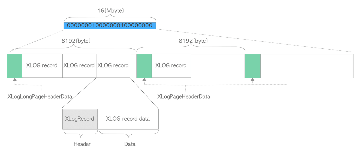
XLOG Record Structure
All XLOG records have a general header portion defined by the XLogRecord structure:
typedef struct XLogRecord
{
        uint32          xl_tot_len;             /* total len of entire record */
        TransactionId   xl_xid;                 /* transaction id */
        XLogRecPtr      xl_prev;                /* ptr to previous record in log */
        uint8           xl_info;                /* flag bits */
        RmgrId          xl_rmid;                /* resource manager for this record */
        /* 2 bytes of padding here, initialize to zero */
        pg_crc32c       xl_crc;                 /* CRC for this record */
        /* XLogRecordBlockHeaders and XLogRecordDataHeader follow, no padding */
} XLogRecord;
The xl_rmid and xl_info fields identify which resource manager should handle the record. Resource managers are collections of operations that define how XLOG records are written and replayed during recovery.
As of recent versions PostgreSQL includes the following resource managers:
| Operation | Resource Manager |
|---|---|
| Heap tuple operations | RM_HEAP, RM_HEAP2 |
| Index operations | RM_BTREE, RM_HASH, RM_GIN, RM_GIST, RM_SPGIST, RM_BRIN |
| Sequence operations | RM_SEQ |
| Transaction operations | RM_XACT, RM_MULTIXACT, RM_CLOG, RM_XLOG, RM_COMMIT_TS |
| Tablespace operations | RM_SMGR, RM_DBASE, RM_TBLSPC, RM_RELMAP |
| Replication and hot standby operations | RM_STANDBY, RM_REPLORIGIN, RM_GENERIC_ID, RM_LOGICALMSG_ID |
Here are representative examples of how resource managers work:
-
When an INSERT statement is issued, the header variables
xl_rmidandxl_infoare set to RM_HEAP and XLOG_HEAP_INSERT, respectively. During recovery, the RM_HEAP resource manager calls itsheap_xlog_insert()function to replay this XLOG record. -
For an UPDATE statement,
xl_infois set to XLOG_HEAP_UPDATE, and theheap_xlog_update()function replays the record during recovery. -
When a transaction commits,
xl_rmidandxl_infoare set to RM_XACT and XLOG_XACT_COMMIT, respectively, and thexact_redo_commit()function replays the record during recovery.PostgreSQL changed its XLOG record structure in version 9.5, introducing a common format that all resource managers can use. This improved maintainability and enables features like WAL compression, which compresses full-page images to save disk space.
While compression does require additional CPU resources during logging, it reduces I/O overhead and WAL file consumption, making it worthwhile for databases with heavy write workloads.
WAL Writer Process
The WAL writer is a background process that periodically checks the WAL buffer and writes all unwritten XLOG records to WAL segment files. This prevents bottlenecks that could occur when large amounts of data are committed simultaneously.
The WAL writer is enabled by default and cannot be disabled. It checks the buffer at intervals specified by the wal_writer_delay parameter, which defaults to 200 milliseconds.
Checkpoint Processing
A checkpoint is a crucial maintenance operation that occurs periodically to prepare the database for recovery and clean up memory.
Checkpoints are triggered when:
- The interval time specified by
checkpoint_timeout(default 300 seconds) has elapsed since the previous checkpoint. - The total size of WAL segment files exceeds the
max_wal_sizethreshold (default 1 GB). - The server shuts down.
- A superuser manually issues the CHECKPOINT command.
When a checkpoint starts, PostgreSQL performs the following steps:
- Records the REDO point—the location where recovery should begin.
- Flushes all data from shared memory to storage.
- Gradually writes all dirty pages from the buffer pool to disk.
- Writes a checkpoint record to the WAL containing the REDO point and other critical information.
- Updates the
pg_controlfile with the latest checkpoint location and metadata.
The pg_control File
The pg_control file is essential for recovery, it is the database's record of where the last checkpoint occurred. It stores fundamental information including the location of the latest checkpoint record, the database state at that time, and transaction IDs needed for recovery.
If the pg_control file becomes corrupted, PostgreSQL cannot start recovery because it lacks a reference point. This makes it one of the most critical files in the database cluster.
Conclusion
Now that the groundwork is laid, the natural next step is understanding how TimescaleDB builds on PostgreSQL to handle high-frequency time series data more efficiently. We'll get into that in the next post.